Modeling Time-Series Data in ClickHouse MergeTree

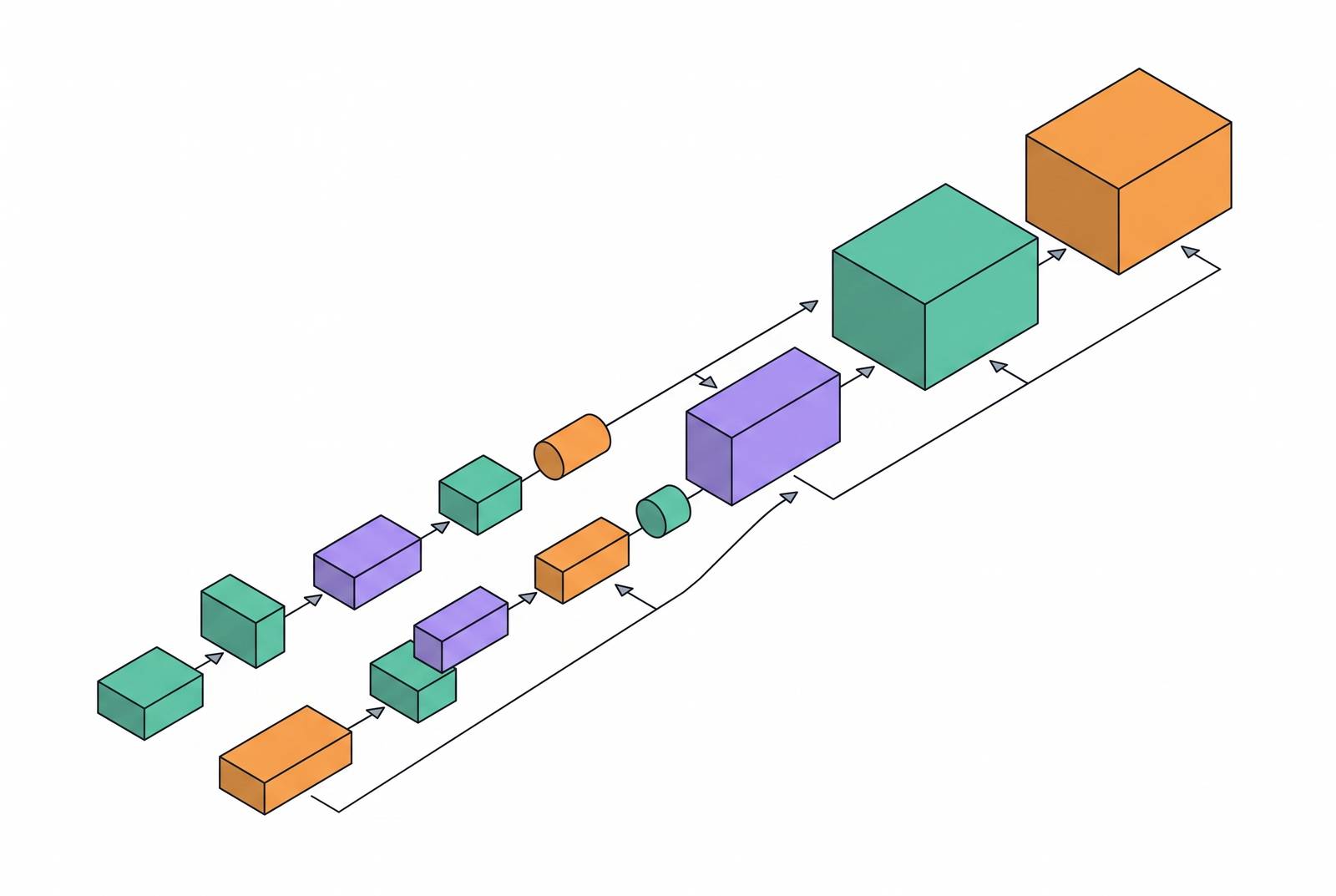
ClickHouse stores time-series data the way it was built to: as columns, appended in bulk, rarely updated. Metrics, logs, events, and sensor readings all share the same shape (a timestamp, a handful of tags, a numeric value, arriving in the millions per hour), and that shape is what ClickHouse's storage engine was designed around from the start. The engine responsible for most of that work is MergeTree, and how you configure it, not just that you use it, decides whether queries return in milliseconds or grind through gigabytes they didn't need to touch.

MergeTree writes each insert as a new, immutable part on disk, then merges those parts in the background into larger, sorted structures. That sorted-parts model is the reason range scans and aggregations run fast on ClickHouse, but the speed appears only when the sort order matches how you actually query the data. Get it wrong, and MergeTree ends up scanning far more than it should. A 100-million-row dataset that takes roughly 100 GiB in PostgreSQL fits in a small fraction of that space in ClickHouse, something like a substantial gap before a single schema decision has even been made. Everything below is about the decisions that build on top of that baseline.

How MergeTree's sparse primary index and granules work

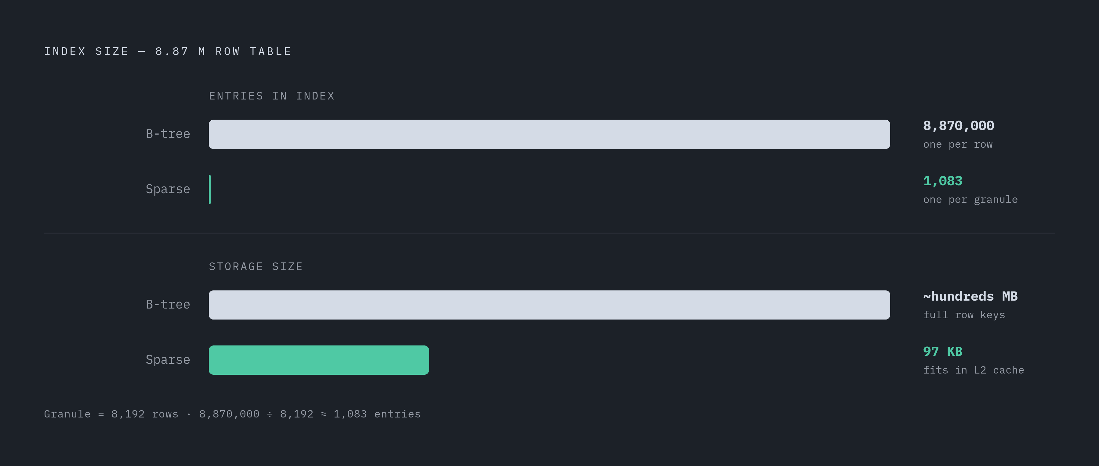
The granule is the smallest chunk of data ClickHouse pulls off disk, 8,192 rows by default, and the primary index holds one entry per granule rather than one per row. That's the "sparse" part: the index isn't trying to point at every row, just at the boundaries of each block.

A query runs a binary search against that index to find which granules could possibly contain matching rows, then reads only those granules, in parallel, off disk. Everything else gets skipped without ever being opened. This only works because the rows inside each part are physically sorted by the primary key already, so a range of values in that key corresponds to a contiguous stretch of rows on disk, not rows scattered across the table. A B-tree, by contrast, has to index every row individually because it has no such guarantee about physical layout.

The size difference this produces is not subtle. On a table with 8.87 million rows, a conventional B-tree index needs 8.87 million entries, easily hundreds of megabytes. ClickHouse's sparse index over the same data needs about 1,083 entries, on the order of 97 KB. That index fits in memory without effort, and it keeps fitting in memory as the table grows into the billions or trillions of rows, because its size tracks the row count divided by the granule size, not the row count itself.

Choosing the ORDER BY key

If there's one schema decision that deserves more design time than the rest combined, it's ORDER BY. Everything downstream, index skipping, merge behavior, compression ratio, hangs off this one choice.

The rule of thumb is to order columns from lowest cardinality to highest, with the columns you filter on most placed leftmost. In a multi-tenant system, that might mean tenant_id comes first, since it's low-cardinality and nearly every query filters on it. After that come progressively higher-cardinality dimensions: site_id, source_id, group_id, maybe a rounded time bucket. The timestamp itself goes last. That placement feels counterintuitive for time-series data until you consider what it buys: putting the timestamp last keeps all the rows for a given series physically near each other on disk, so a query for "this host, this metric, over this time range" reads one contiguous block instead of scattering across the whole table.

The contrast is visible clearly in practice. An ORDER BY of (host, metric, ts) lets a query filtering on host and metric skip straight to the relevant granules. An ORDER BY of (ts) alone does close to the opposite: every series gets interleaved by time, so pulling the history of one host means touching nearly every part in the table, which turns a targeted query into a full scan.

ClickHouse treats PRIMARY KEY and ORDER BY as related but distinct. The primary key has to be a prefix of the ORDER BY columns, and it's what actually drives physical sort order and granule skipping. ORDER BY can extend beyond the primary key with extra columns that don't help with skipping but do matter for other things, deduplication in ReplacingMergeTree being the clearest example.

Picking timestamp and dimension data types before any codec is applied

Type selection happens before codec selection, and it deserves its own decision, separate from compression tuning. Get the type wrong and no codec fixes it after the fact.

For timestamps, ClickHouse offers a small ladder of precision and cost. Date takes 2 bytes and covers 1970 through 2149, which is plenty if you only need day-level granularity. DateTime takes 4 bytes at one-second precision, and that's the right choice for most metrics workloads, both because a second is usually fine and because it compresses better than the higher-precision types. DateTime64(3) moves to millisecond precision at 8 bytes, useful when events genuinely happen sub-second apart. DateTime64(9) goes to nanosecond precision, also at 8 bytes, and that's a niche for high-frequency trading systems or sensor logging where nanosecond fidelity actually matters to someone downstream. Version 25.6 added Time/Time64 types for storing a time-of-day value with no date component; using them requires setting enable_time_time64_type = 1, and they don't carry timezone information.

Timezones themselves are worth a specific callout. Without an explicit timezone in the column definition, ClickHouse writes using the server's local timezone. Attaching a timezone directly to the column, DateTime('Europe/Berlin'), for instance, triggers automatic conversion on insert. For anything spanning multiple regions, getting that distinction wrong turns a clean dataset into a quietly corrupted one.

Dimension columns follow a separate logic. Any field with fewer than roughly 10,000 distinct values, host names, region codes, metric names, HTTP status categories, is a strong candidate for LowCardinality(String), which triggers dictionary encoding under the hood: the engine stores small integer references instead of repeating string values, and both I/O and GROUP BY performance benefit. High-cardinality string fields, log messages, UUIDs, free text, are better left as plain String with a ZSTD codec, since dictionary encoding doesn't help when nearly every value is unique. Numeric columns should use the smallest integer type that actually fits the data: UInt16 for an HTTP status code, UInt64 for a counter, and a choice between Float32 and Float64 based on how much precision the value genuinely needs.

Choosing the right data type, independent of any codec applied on top, can cut storage by something on the order of 12% and cut query time by around half.

Column codecs

Compression in ClickHouse happens in two stages. First an encoding codec transforms the data to reduce its entropy (this step, on its own, doesn't shrink anything), and then a byte-level compressor, LZ4 or ZSTD, actually squeezes the transformed bytes down. Codecs can be chained in the column definition, and for time-series data, matching the right encoding codec to the right column type is where most of the compression gain lives.

DoubleDelta is the standard choice for timestamps. It stores second-order differences, the delta of the deltas, which works exceptionally well on monotonic sequences with a roughly constant stride, which is what a regular timestamp column looks like. Reported compression on timestamp columns using DoubleDelta runs several times over to well over an order of magnitude. Delta, the simpler first-order version, suits monotonically increasing integers like counters or sequence numbers better than it suits timestamps, since it doesn't account for the constant-stride pattern that DoubleDelta exploits.

For floating-point gauges, Gorilla is the established codec: it XORs each value against the previous one, then encodes the leading and trailing zero bits of that XOR, exploiting the fact that consecutive readings in a time series tend to be close in value. The technique traces back to Facebook's original Gorilla work, which reported a substantial reduction on production time-series data; on smooth float gauges more generally, the range typically runs from several times over to roughly an order of magnitude. Gorilla remains the established choice for float columns, and existing schemas running it don't need revisiting unless a broader schema change is already underway. T64 rounds out the set, stripping unused high bits from integer columns with a narrow actual range.

On the byte-compressor side, LZ4 is the default and decodes fastest, making it the right pairing when query latency is the priority. ZSTD, tunable by level as ZSTD(n), trades more CPU on decode for a better compression ratio, which makes it the better fit for cold columns or data that's mostly sitting in archival storage.

One pairing is worth avoiding: chaining Delta or DoubleDelta with Gorilla adds overhead without real compression benefit, because Gorilla already performs an implicit delta step internally.

Partitioning granularity: a data management tool, not a query optimization shortcut

ClickHouse's own documentation is direct about this: partitioning exists mainly as a data management mechanism, not a way to speed up queries. Reaching for partitioning first when a query is slow is usually a misdiagnosis. It's ORDER BY, not partition key, that governs query-time granule skipping.

What partitioning actually delivers is operational. It splits data into separate physical directories by the partition key. A whole partition can be dropped in one ALTER TABLE ... DROP PARTITION statement instead of deleting rows one at a time. For time-series retention, that's the entire point: dropping a month or a day of expired data becomes a metadata operation instead of a scan-and-delete job.

Sizing matters here. Partitions in the range of 10 GB to 1 TB each tend to work well; go much smaller and you end up with too many small parts for MergeTree to manage efficiently, go much bigger and you lose the operational flexibility partitioning was supposed to provide. Monthly partitioning, toYYYYMM(ts), is a reasonable default for most workloads. Daily partitioning, toYYYYMMDD(ts), suits higher-volume data with shorter retention windows. Hourly partitioning belongs only to genuinely very high-volume cases. Composite partition keys, month plus region, or date plus tenant_id, are supported, but they need care: stacking too many dimensions into the partition key multiplies the number of partitions and tends to degrade performance rather than help it.

TTL rules: automating retention and tiering without manual intervention

TTL rules in MergeTree can operate at the row level or the table level, and for time-series data, the standard pattern is a table-level TTL tied directly to the timestamp column.

TTL expiration is evaluated during background merges, not the instant a row crosses its expiration threshold. Data that's aged out sits on disk until the next merge cycle touches that part. That's a deliberate design choice, not an oversight, and it means retention isn't instantaneous, it's eventual, on the same timescale as the rest of MergeTree's background work.

The basic syntax is simple: TTL ts + INTERVAL 1 YEAR drops rows older than a year once a merge processes their part. TTL also supports tiering, not just deletion: TTL ts + INTERVAL 30 DAY TO DISK 'cold' moves data older than 30 days to a separate, cheaper storage volume automatically. That's a hot/warm/cold storage architecture built entirely into the table definition, with no application code deciding when to move data around.

Putting the decisions together: a minimal schema and a multi-dimensional extension

All of the above converges into something that can be surprisingly small. A minimum viable time-series table in ClickHouse needs only three columns:

CREATE TABLE metrics (
    series_id UInt32 CODEC(LZ4),
    ts DateTime CODEC(DoubleDelta, LZ4),
    value Float64 CODEC(Gorilla, LZ4)
)
ENGINE = MergeTree()
PARTITION BY toYYYYMM(ts)
ORDER BY (series_id, ts)
TTL ts + INTERVAL 1 YEAR
SETTINGS index_granularity = 8192

Every piece here maps back to a decision made earlier: series_id leads the ORDER BY because it's the low-cardinality filter column, ts trails it and carries DoubleDelta because it's a near-constant-stride sequence, value carries Gorilla because it's a float gauge, and the TTL clause handles a year of retention without a scheduled job anywhere in sight.

Real workloads add columns beyond this, host, region, status code, and each one should go through the same series of decisions rather than being bolted on by default: does it belong in ORDER BY, what's its cardinality, does it need LowCardinality(String), what codec fits its actual data pattern. Every additional column is overhead against the compression and scan efficiency this schema is built to protect, so the discipline is to add only what the query patterns actually require, not what might someday be useful.