Reading ClickHouse EXPLAIN Plans for Query Tuning

ClickHouse runs every query through four phases: parsing and analysis, optimization, pipeline execution, and final formatting. Each one hands off to the next, and each one can hide a different kind of mistake. EXPLAIN is the tool for catching those mistakes, but it isn't one tool so much as several, and picking the wrong variant means staring at the wrong layer entirely.

Consider that before touching a single query. Because ClickHouse stores data by column and indexes it sparsely rather than row by row, whether a query takes ten milliseconds or ten seconds gets decided before a single value is decompressed. By the time results come back, the outcome was already fixed several phases earlier. Reading the plan is how you find out, ahead of time, whether the fix belongs in the schema, the query itself, or the indexing layer. You won't know which until you look.

The full family of EXPLAIN variants and what layer each one targets

The full syntax is EXPLAIN, followed by one of several keywords (AST, SYNTAX, QUERY TREE, PLAN, PIPELINE, ANALYZE, ESTIMATE, TABLE OVERRIDE, WHATIF), optional settings, then the query itself. Each keyword corresponds to a different stage of query processing, and that's by design rather than an accident of the API.

SYNTAX shows the query text after AST-level rewrites, so you can see what the optimizer changed before it ever built a plan. QUERY TREE shows the analyzer's internal representation after its own optimization pass, and it's the one to reach for when something behaves differently across ClickHouse versions and you suspect the analyzer is doing something new. PLAN is the logical execution plan, a tree of named steps, and it's the workhorse for most day-to-day tuning. PIPELINE goes one level deeper still, showing the actual processor graph and thread counts that will run on the box. ESTIMATE gives you row, mark, and part counts without running anything, a pre-flight check. ANALYZE, new as of version 26.7, actually executes the query and annotates the plan with measured runtime numbers rather than estimates. WHATIF, added in version 26.6, lets you test a hypothetical skip index without materializing it on disk.

As a rough decision guide: start most slow-query investigations with PLAN plus indexes = 1. Reach for PIPELINE when CPU utilization looks off. Use ESTIMATE for a quick cost check before running something expensive. Use WHATIF before committing disk space and write overhead to a new skip index. And use ANALYZE when you need actual timing, not a guess.

EXPLAIN with no keyword at all defaults to PLAN. A lot of examples floating around online omit the keyword entirely, which is fine, but knowing what you're actually looking at matters.

Reading EXPLAIN PLAN: the node tree, how data flows through it, and what each node signals

A plan reads as a tree, and the convention takes some getting used to: data enters at the innermost node, the leaf, and each layer above it transforms the stream further until it reaches the top, which is what gets handed back to the client.

For a typical query with GROUP BY, ORDER BY, and LIMIT, the node sequence from top to bottom looks roughly like this: Projection, then Limit, then Sorting, then an intermediate expression step, then Aggregating, another expression step, a Filter for the WHERE clause, and finally ReadFromMergeTree at the very bottom. That last node is the leaf, the place where actual data gets pulled off disk, and it's where most of the wins and losses in a query get decided.

ReadFromMergeTree names the table being scanned and reports a ReadType. ReadFromMergeTree names the table being scanned and reports a ReadType. Default means a standard, unordered, parallel read. InOrder means ClickHouse is reading in primary-key order, which is a strong performance signal when your ORDER BY happens to match that key. InReverseOrder is the same idea run backward.

Filter nodes show up when a predicate couldn't be pushed down into storage and has to run separately. Where that Filter sits in the tree affects performance far more than whether it exists at all. A Filter sitting right above ReadFromMergeTree is fine, it's filtering close to the source. A Filter sitting above an Aggregating step or a Join, though, is a signal worth investigating, since it may indicate that filtering is happening later in the pipeline than ideal. That's visible in the plan before you ever run the query.

An Aggregating step can sit directly above ReadFromMergeTree, with no Filter or expression step between them. That usually means partial aggregation is happening at the storage level itself, because the aggregation key lines up with the table's sort order. It's a genuine performance win, and it's the kind of thing you'd never notice without looking at the tree directly.

A handful of settings change how much detail PLAN prints. header = 1 shows column names and types at each step. description = 1 is on by default and prints a short description per step. actions = 1 shows the detailed operations at each node. And indexes = 1, the most important of the four, is worth its own section.

EXPLAIN indexes = 1: the Parts and Granules ratio as the primary diagnostic for MergeTree scans

ClickHouse's primary index isn't dense. It stores one entry per 8,192 rows, a unit called a granule, rather than one entry per row. On a table with a large number of rows, that works out to a modest number of index entries, a small total size, small enough to sit comfortably in memory no matter how large the table grows.

The tradeoff for that compactness is that granules are the smallest unit ClickHouse can skip. If even one row inside a granule matches a filter, the engine has to read all 8,192 rows in that granule, whether nearly all the rest are relevant or not. At worst, a value sitting right on a granule boundary can force ClickHouse to read up to 16,384 rows to satisfy a match on a single one. That's not a defect in the engine. It's the ceiling cost of resolving matches at granule granularity instead of row granularity, and it's a fair trade for keeping the index small enough to hold in memory at any scale.

EXPLAIN indexes = 1 shows how well that granule-skipping worked for a given query. It adds three things to the output: a Parts line (parts read over total parts), a Granules line (granules read over total granules), and a PrimaryKey block showing which key columns the optimizer actually used and what condition it applied.

The Granules ratio is the number to watch first. Something like Parts: 3/12, Granules: 41/980 describes a query that pruned aggressively, touching a small slice of the table. A ratio like Granules: 5/122000 is close to ideal, over 99.99% of granules never got touched. Compare that to Parts: 892/892, Granules: 45231/45231, where every part and every granule got read. That's a full scan, and it almost always means the WHERE clause isn't using the primary key at all, whatever the schema's key column order might suggest.

The three-layer pruning architecture visible in EXPLAIN output: partition, primary index, skip indexes

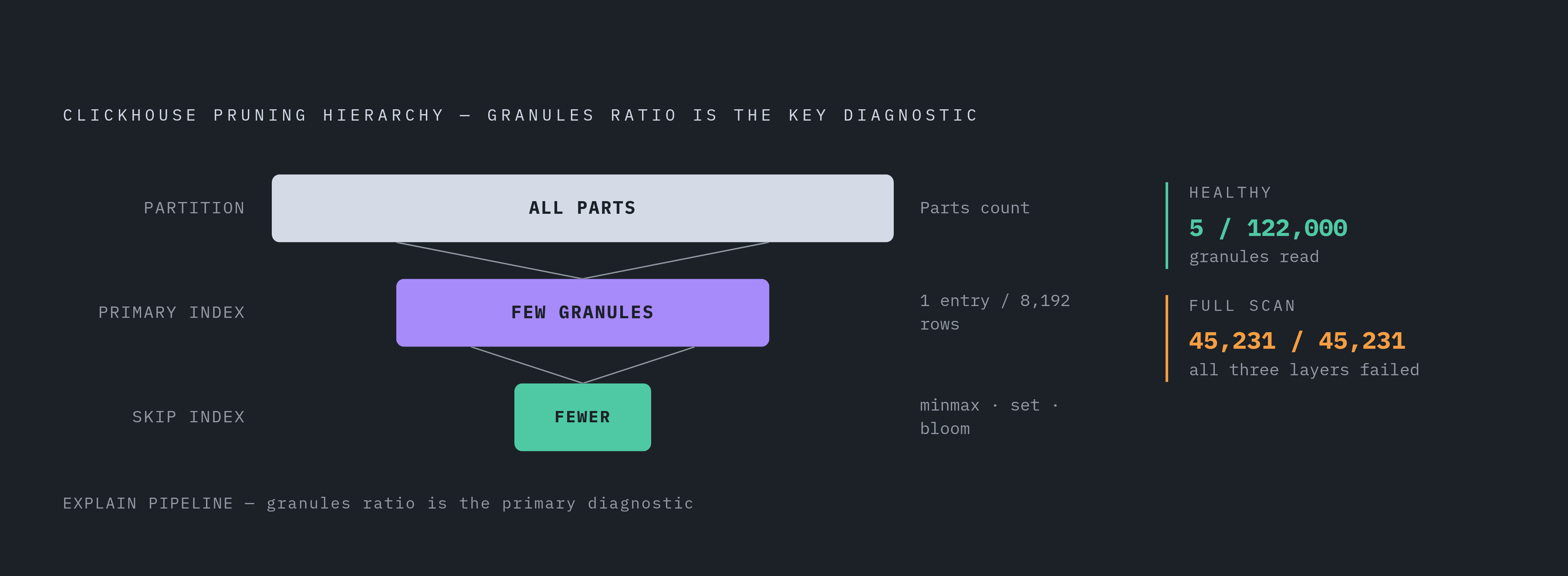
ClickHouse prunes data in three passes, moving from coarse to fine. Partition pruning comes first and eliminates entire partitions outright, the biggest chunks available. A Parts count that's already small before the primary key logic has done anything at all appears in EXPLAIN.

Next comes the primary index itself, the sparse structure described above, which eliminates granules that fall outside the sorted key range. This is what the Granules ratio measures directly. Last comes any skip index defined on the table, which narrows further within whatever range the primary index couldn't already exclude.

Run together, these three layers can take a query from reading nearly all of a table's data down to a tiny fraction, and EXPLAIN indexes = 1 is the one command that shows all three layers doing their work in a single pass. The way to read it: check Parts first, since that's partition pruning. Then compare the Granules ratio before and after the primary key condition to gauge how much the sparse index bought you. Then check whether a skip index block appears at all and how many further granules it removed.

If partition pruning looks fine but the Granules ratio is still near 100%, the real fix usually lies in the ordering of columns in the primary key, or a rewrite of the query to filter on columns that key actually covers. It's the ordering of columns in the primary key, or a rewrite of the query to filter on columns that key actually covers. If Granules are partially pruned but still uncomfortably high after that, that's the case where a skip index earns its keep.

Skip indexes: what the five types cover, how EXPLAIN validates them, and the write-cost tradeoff

ClickHouse ships several types of skip index, and each one targets a different filter shape. minmax suits range filters on columns whose values change slowly as you move through sort order. set handles equality filters on low-cardinality columns. bloom_filter covers exact-match membership checks on strings and arrays. ngrambf_v1 is built for substring and full-text search. tokenbf_v1 handles token or word-level search.

Bloom filters work by checking, at query time, whether a granule could possibly contain a match before ClickHouse bothers reading it. They never produce a false negative, so no matching row ever gets silently skipped, but they can produce false positives, occasionally sending the engine to scan a granule that turns out not to match after all. That tradeoff keeps the index small on disk while still cutting a large share of unnecessary I/O.

The magnitude of that gain is not theoretical. In one measured case, attribute-based trace search ran roughly 40 times slower than every other query type it was compared against, 1,769 milliseconds against a range of 37 to 47 milliseconds. The cause traced back to arrayExists calls with no skip index in place, which forced ClickHouse to decompress and scan every single granule regardless of relevance. Adding bloom filter skip indexes on the relevant columns closed that gap.

Bloom-style indexes are most effective for positive membership checks rather than negated predicates, because a bloom filter can confirm a possible match but can't reliably confirm an absence of one, so this needs to be planned around from the start. That's a schema-design decision, not something EXPLAIN alone will fix after the fact.

EXPLAIN SYNTAX and EXPLAIN QUERY TREE: catching optimizer rewrites before they cause confusion

EXPLAIN SYNTAX prints the query as it looks after AST-level rewrites, and it's the fastest way to confirm whether the optimizer did what you expected: pushed a predicate down, rewrote an IN subquery, or, just as usefully, failed to apply an optimization you assumed it would.

Check whether a WHERE condition moved into PREWHERE. When it does, the optimizer decided that condition was cheap and selective enough to filter early, before reading the rest of the row. When a condition you expected to move didn't, investigate it, and sometimes the fix is as simple as adding it to PREWHERE by hand rather than trusting the optimizer to find it.

EXPLAIN QUERY TREE serves a related but distinct purpose. It exposes the analyzer's own internal representation after its optimization pass, and it's most useful on newer versions of the database engine when you're trying to understand analyzer-specific behavior that doesn't map cleanly onto the older tree-based view.

Run EXPLAIN SYNTAX before diving into EXPLAIN PLAN on any slow query. If the rewritten query looks nothing like what was actually typed, everything downstream in the plan describes the rewritten version, not the original. Skipping that check is a reliable way to misdiagnose a problem that isn't where you think it is.

EXPLAIN PIPELINE: reading thread counts, parallelism, and the Resize bottleneck

PIPELINE is the deepest layer available, showing the actual physical execution graph, the real streams of data ClickHouse spins up to run the query, rather than the logical steps described in PLAN.

The notation takes a moment to parse. A "× N" next to a processor means N parallel threads are working that stage simultaneously, and N is governed by the max_threads setting, which defaults to the number of CPU cores available on the box.

Three things need checking specifically in this output. First, the thread count on MergeTreeThread processors: seeing a bare 1 there means the query isn't spreading across available cores at all, and the fix starts with the max_threads setting. Second, look for a Resize step in the graph, which shows where multiple parallel streams of partial work get funneled down into fewer threads to finish the job, and that funnel point is where overall throughput can cap out no matter how much parallel work happened upstream. Third, consider the memory cost of parallelism itself: each thread holds its own buffers, so high thread counts combined with wide aggregations can push memory pressure up quickly, another dial controlled through max_threads.

PIPELINE earns its place in the workflow specifically when PLAN looks reasonable but the wall-clock time doesn't match what the plan implies, when a query seems to be ignoring the cores it should have access to, or when an aggregation is suspected of running single-threaded despite a machine with plenty of headroom to spare. In each of those cases, PLAN alone won't show the problem, because the problem doesn't live in the logical steps. It lives in how those steps got wired into actual threads, and that's a layer only PIPELINE exposes.